Sakthi Swaroopan S - CB.BU.P2ASB25147
0) Setup
# install.packages(c("readxl","dplyr","magrittr","factoextra","rattle","DT","psych","tibble","tidyr"))


library(readxl)
library(dplyr)
library(magrittr)
library(factoextra)
library(rattle)
library(DT)
library(psych)
library(tibble)
library(tidyr)


set.seed(42)


# ---- Paths ----
DATA_PATH <- "/ESG_Dataset_Sakthi.xlsx"
SHEET_NAME <- "Sheet1"
1) Importing the data
Data was collected through the annual reports sourced from NSE.
raw <- read_excel(DATA_PATH, sheet = SHEET_NAME) %>%
janitor::clean_names() # using janitor fully qualified (not attaching)


# Expected columns after clean_names():
# company_name, year, industry_type, ceo_name, ceo_gender,
# carbon_emissions, energy_consumption, employee_turnover, roe, roa
2) Exploratory analysis
# Structure and a peek
str(raw)
## tibble [48 × 11] (S3: tbl_df/tbl/data.frame)
##  $ company_name      : chr [1:48] "Sona BLW Percision forgings ltd" "Sona BLW Percision forgings ltd" "Sona BLW Percision forgings ltd" "Sona BLW Percision forgings ltd" ...
##  $ year              : num [1:48] 2021 2022 2023 2024 2025 ...
##  $ carbon_emissions  : chr [1:48] "32756" "40330" "48468" "58317" ...
##  $ energy_consumption: chr [1:48] "41800.07" "52308.14" "311100" "358157" ...
##  $ employee_turnover : chr [1:48] "7.6499999999999999E-2" "0.11" "0.16" "0.13" ...
##  $ roa               : num [1:48] 0.1065 0.141 0.1303 0.1351 0.0941 ...
##  $ roe               : num [1:48] 0.153 0.179 0.172 0.188 0.107 ...
##  $ industry_type     : chr [1:48] "Automotive" "Automotive" "Automotive" "Automotive" ...
##  $ location          : chr [1:48] "Haryana" "Haryana" "Haryana" "Haryana" ...
##  $ ceo_name          : chr [1:48] "Vivek Vikram Singh" "Vivek Vikram Singh" "Vivek Vikram Singh" "Vivek Vikram Singh" ...
##  $ ceo_gender        : chr [1:48] "Male" "Male" "Male" "Male" ...
DT::datatable(head(raw, 20), options = list(pageLength = 10), caption = "Raw data (first 20 rows)")
## Error in loadNamespace(name): there is no package called 'webshot'
# Simple counts
raw %>% count(company_name, sort = TRUE) %>% DT::datatable(caption = "Rows per company")
## Error in loadNamespace(name): there is no package called 'webshot'
raw %>% count(year, sort = TRUE) %>% DT::datatable(caption = "Rows per year")
## Error in loadNamespace(name): there is no package called 'webshot'
3) Pre‑processing the data
Rules applied
-
Drop rows where Energy_Consumption == “Not Reported”. This ensures comparability between the companies.
-
Replace NA in Carbon_Emissions with 0 for non-manufacturing firms.
-
Cast types for numeric columns; keep factors for categories.
-
Standardizing Decimals to improve readability and consistency.
df <- raw %>%
# Normalize text placeholders to real NAs
mutate(
energy_consumption = dplyr::na_if(energy_consumption, "Not Reported"),
carbon_emissions = dplyr::na_if(carbon_emissions, "NA")
) %>%
# Coerce to appropriate types
mutate(
year = as.integer(year),
industry_type = as.factor(industry_type),
ceo_gender = factor(ceo_gender, levels = c("Male","Female","Other")),
energy_consumption = suppressWarnings(as.numeric(energy_consumption)),
carbon_emissions = suppressWarnings(as.numeric(carbon_emissions)),
employee_turnover = suppressWarnings(as.numeric(employee_turnover)),
roe = suppressWarnings(as.numeric(roe)),
roa = suppressWarnings(as.numeric(roa))
) %>%
# Apply the two cleaning rules
filter(!is.na(energy_consumption)) %>% # drop Not Reported rows
mutate(carbon_emissions = dplyr::coalesce(carbon_emissions, 0)) %>%
mutate(across(c(carbon_emissions, energy_consumption,employee_turnover, roe, roa), ~ round(.x, 2))) %>%
arrange(company_name, year)


# Quick sanity check
stopifnot(all(c("company_name","year","industry_type","ceo_gender",
"carbon_emissions","energy_consumption","employee_turnover","roe","roa") %in% names(df)))
4) Preview of data before analysis
DT::datatable(head(df, 20), options = list(pageLength = 10), caption = "Cleaned data (first 20 rows)")
## Error in loadNamespace(name): there is no package called 'webshot'
5) Exploratory analysis (post‑clean)
# Numeric summary by year
year_summary <- df %>%
group_by(year) %>%
summarise(
n = dplyr::n(),
mean_emissions = mean(carbon_emissions, na.rm = TRUE),
mean_energy = mean(energy_consumption, na.rm = TRUE),
mean_turnover = mean(employee_turnover, na.rm = TRUE),
mean_roe = mean(roe, na.rm = TRUE),
mean_roa = mean(roa, na.rm = TRUE)
)
DT::datatable(year_summary, caption = "Year‑wise summary")
## Error in loadNamespace(name): there is no package called 'webshot'
# Correlation matrix (pooled numeric)
num_cols <- c("carbon_emissions","energy_consumption","employee_turnover","roe","roa")
cor_mat <- stats::cor(df[, num_cols], use = "pairwise.complete.obs")
cor_mat <- round(cor_mat, 2)
cor_mat
##                    carbon_emissions energy_consumption employee_turnover   roe   roa
## carbon_emissions               1.00              -0.15             -0.46  0.03  0.13
## energy_consumption            -0.15               1.00              0.04 -0.22 -0.14
## employee_turnover             -0.46               0.04              1.00 -0.24 -0.22
## roe                            0.03              -0.22             -0.24  1.00  0.94
## roa                            0.13              -0.14             -0.22  0.94  1.00
# helper function to convert psych::describe output into vertical key-value tibble
describe_long <- function(x) {
  psych::describe(x) %>%
    as_tibble() %>%
    select(-vars, -n) %>%   # drop unneeded cols (keep stats)
    pivot_longer(cols = everything(),
                 names_to = "Metric",
                 values_to = "Value")
}

# Now display each variable as vertical DT
DT::datatable(describe_long(df["carbon_emissions"]), caption = "Carbon Emissions")
## Error in loadNamespace(name): there is no package called 'webshot'
DT::datatable(describe_long(df["energy_consumption"]), caption = "Energy Consumption")
## Error in loadNamespace(name): there is no package called 'webshot'
DT::datatable(describe_long(df["employee_turnover"]), caption = "Employee Turnover")
## Error in loadNamespace(name): there is no package called 'webshot'
DT::datatable(describe_long(df["roe"]), caption = "ROE")
## Error in loadNamespace(name): there is no package called 'webshot'
DT::datatable(describe_long(df["roa"]), caption = "ROA")
## Error in loadNamespace(name): there is no package called 'webshot'
- Energy consumption and emissions remain volatile, without a steady downward trend.
6) Analysis
company_summary <- df %>%
  group_by(company_name) %>%
  summarise(
    avg_emissions   = mean(carbon_emissions, na.rm = TRUE),
    avg_energy      = mean(energy_consumption, na.rm = TRUE),
    avg_turnover    = mean(employee_turnover, na.rm = TRUE),
    avg_roe         = mean(roe, na.rm = TRUE),
    avg_roa         = mean(roa, na.rm = TRUE),
    .groups = "drop"
  ) %>%
  arrange(desc(avg_roe))

DT::datatable(
  company_summary,
  caption = "5-Year Company Performance Snapshot (Averages)",
  options = list(pageLength = 10)
)
## Error in loadNamespace(name): there is no package called 'webshot'
Some firms balance profitability with efficiency, while others underperform despite high energy/emissions.
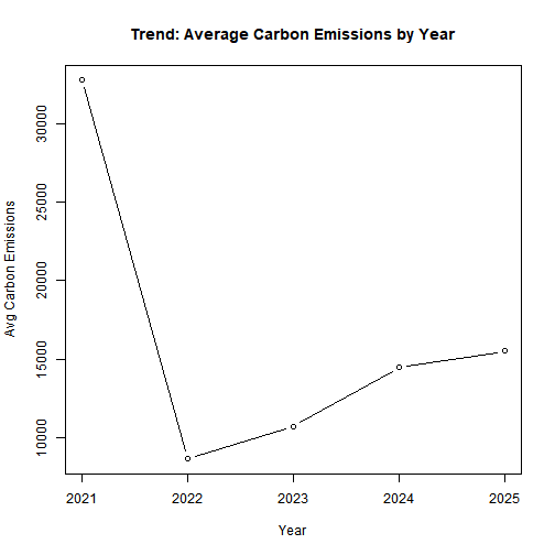
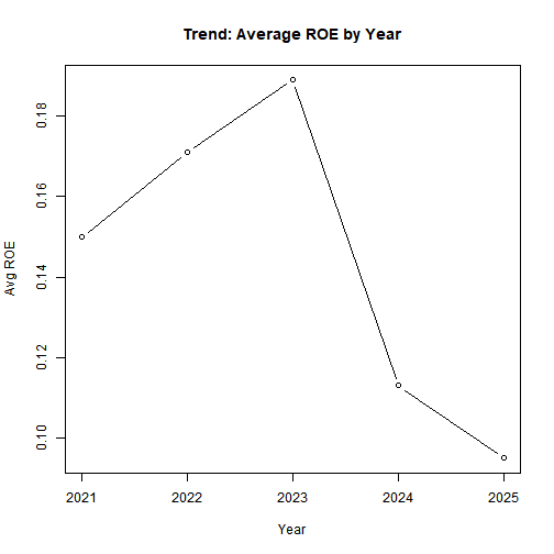
6.2) Year-over-year Trends
# Recompute to keep the section self-contained
yoy <- df %>%
  group_by(year) %>%
  summarise(
    mean_emissions = mean(carbon_emissions, na.rm = TRUE),
    mean_energy    = mean(energy_consumption, na.rm = TRUE),
    mean_turnover  = mean(employee_turnover, na.rm = TRUE),
    mean_roe       = mean(roe, na.rm = TRUE),
    mean_roa       = mean(roa, na.rm = TRUE),
    .groups = "drop"
  ) %>%
  arrange(year)

DT::datatable(
  yoy,
  caption = "Year-wise Averages (Sustainability & Profitability)"
)
## Error in loadNamespace(name): there is no package called 'webshot'
# Emissions trend
plot(
  yoy$year, yoy$mean_emissions, type = "b",
  xlab = "Year", ylab = "Avg Carbon Emissions",
  main = "Trend: Average Carbon Emissions by Year"
)
# ROE trend
plot(
  yoy$year, yoy$mean_roe, type = "b",
  xlab = "Year", ylab = "Avg ROE",
  main = "Trend: Average ROE by Year"
)
# ROA trend
plot(
  yoy$year, yoy$mean_roa, type = "b",
  xlab = "Year", ylab = "Avg ROA",
  main = "Trend: Average ROA by Year"
)
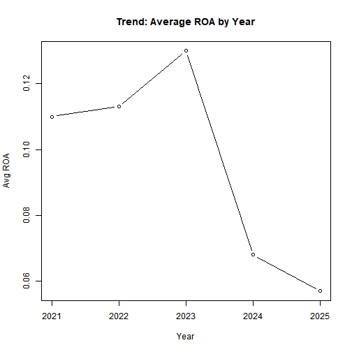
Modest improvement in profitability, but sustainability indicators (emissions, energy) do not show consistent decline.
6.3) Comparative Plots
# Helper to draw scatter + OLS line + correlation
make_scatter <- function(x, y, xlab, ylab, title) {
ok <- is.finite(x) & is.finite(y)
plot(x[ok], y[ok],
xlab = xlab, ylab = ylab,
main = title, pch = 19)
# OLS line
fit <- stats::lm(y[ok] ~ x[ok])
abline(fit, lwd = 2)
# Pearson correlation
r <- stats::cor(x[ok], y[ok], method = "pearson")
legend("topleft", bty = "n",
legend = paste0("r = ", round(r, 2)))
}
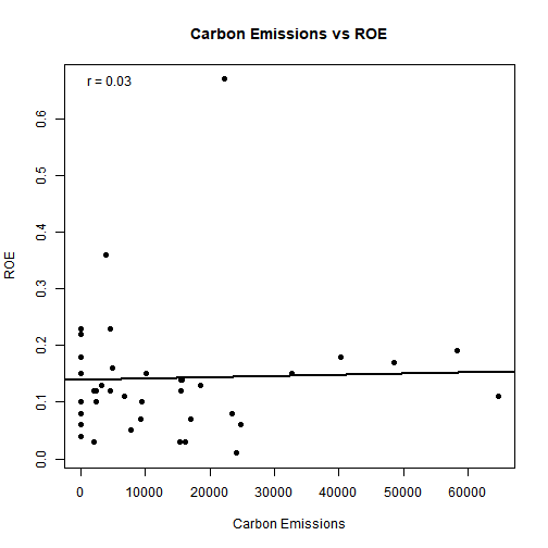
# Emissions vs ROE
make_scatter(
x = df$carbon_emissions, y = df$roe,
xlab = "Carbon Emissions", ylab = "ROE",
title = "Carbon Emissions vs ROE"
)
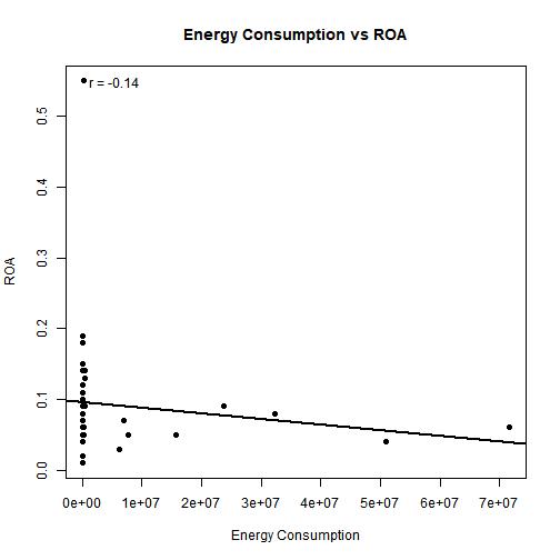
# Energy vs ROA
make_scatter(
  x = df$energy_consumption, y = df$roa,
  xlab = "Energy Consumption", ylab = "ROA",
  title = "Energy Consumption vs ROA"
)
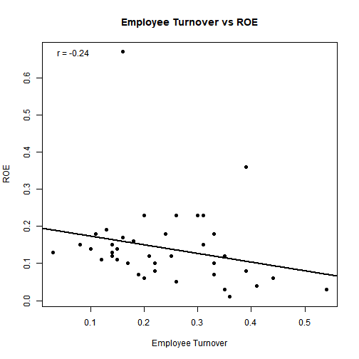
# Turnover vs ROE
make_scatter(
  x = df$employee_turnover, y = df$roe,
  xlab = "Employee Turnover", ylab = "ROE",
  title = "Employee Turnover vs ROE"
)
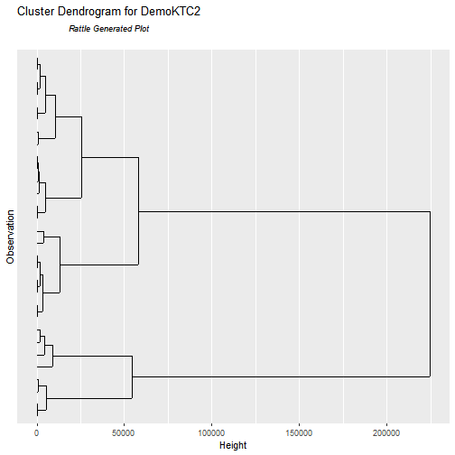
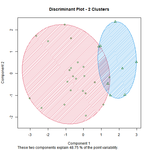
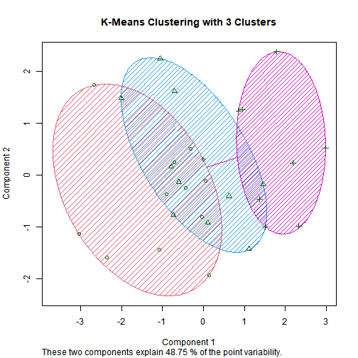
6.4) Clustering
clust_df <- df %>%
  group_by(company_name, industry_type) %>%
  summarise(
    carbon_emissions   = mean(carbon_emissions,   na.rm = TRUE),
    energy_consumption = mean(energy_consumption, na.rm = TRUE),
    employee_turnover  = mean(employee_turnover,  na.rm = TRUE),
    roe                = mean(roe,                na.rm = TRUE),
    roa                = mean(roa,                na.rm = TRUE),
    .groups = "drop"
  )

# Variables used for clustering (inputs)
vars_used <- c("carbon_emissions", "energy_consumption",
               "employee_turnover", "roe", "roa")
DT::datatable(
  tibble::tibble(Variables_Used = vars_used),
  caption = "Variables used for clustering (company-level averages)"
)
## Error in loadNamespace(name): there is no package called 'webshot'
# Prepare numeric matrix and scale
X <- clust_df %>% dplyr::select(all_of(vars_used)) %>% as.data.frame()
X_scaled <- scale(X)
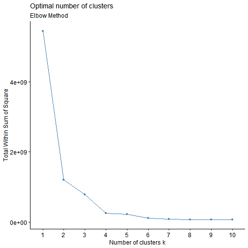
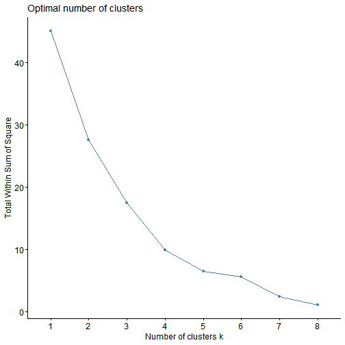
# choose K (WSS / Silhouette)
factoextra::fviz_nbclust(X_scaled, kmeans, method = "wss", k.max = 8)
factoextra::fviz_nbclust(X_scaled, kmeans, method = "silhouette", k.max = 8)
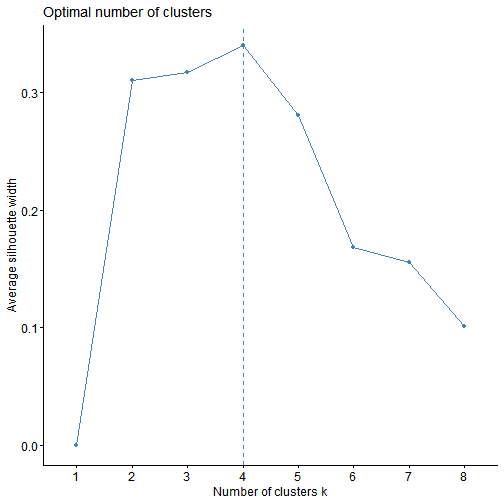
# Fit K-means (set k after inspecting above plots)
k <- 3
km <- stats::kmeans(X_scaled, centers = k, nstart = 50)

# Attach cluster ids to companies
clust_out <- clust_df %>% mutate(cluster = factor(km$cluster))
DT::datatable(clust_out, caption = "Company → Cluster assignments")
## Error in loadNamespace(name): there is no package called 'webshot'
# Companies in each cluster (compact list)
companies_by_cluster <- clust_out %>%
  group_by(cluster) %>%
  summarise(companies = paste(company_name, collapse = ", "), .groups = "drop")
DT::datatable(companies_by_cluster, caption = "Companies in each cluster")
## Error in loadNamespace(name): there is no package called 'webshot'
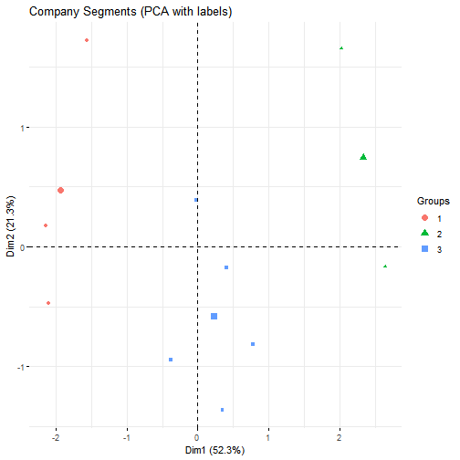
# PCA for labeled visualization (labels = company names)
rownames(X_scaled) <- clust_df$company_name
pca_obj <- stats::prcomp(X_scaled, center = FALSE, scale. = FALSE)  # already scaled

factoextra::fviz_pca_ind(
  pca_obj,
  geom = "point",
  habillage = clust_out$cluster,   # color by cluster
  addEllipses = FALSE,             # avoid ellipse warnings for small clusters
  label = "all",                   # show company labels
  repel = TRUE,                    # nicer label placement
  title = "Company Segments (PCA with labels)"
)
# PCA loadings table to interpret Dim1/Dim2 drivers
loadings <- tibble::as_tibble(pca_obj$rotation[, 1:2], rownames = "variable")
colnames(loadings) <- c("variable", "Dim1_loading", "Dim2_loading")
DT::datatable(loadings, caption = "PCA loadings (which variables drive Dim1/Dim2)")
## Error in loadNamespace(name): there is no package called 'webshot'
# Cluster-level profiles (means of original features)
cluster_profiles <- clust_out %>%
  group_by(cluster) %>%
  summarise(across(all_of(vars_used), ~ mean(.x, na.rm = TRUE)), .groups = "drop")
DT::datatable(cluster_profiles, caption = "Cluster profiles (feature means)")
## Error in loadNamespace(name): there is no package called 'webshot'
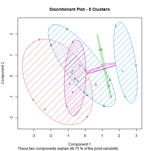
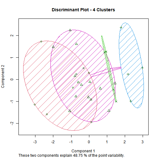
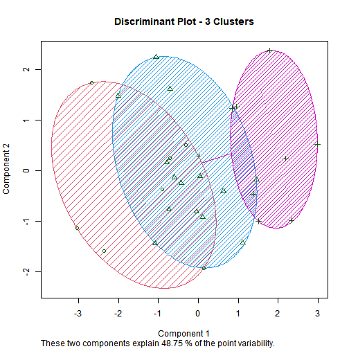
-
Three groups emerge:
-
Efficient & Profitable (low emissions, higher returns).
-
Transitioners (partial improvements).
-
Underperformers (high energy/emissions, low returns).
- Automotive company stands out with both high emissions and high profitability.
6.5) Predictive analysis
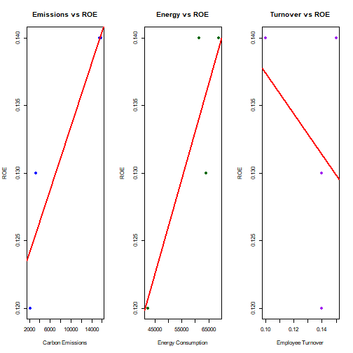
6.5.1) Company-wise Prediction
# Filter company
df_c <- df %>% filter(company_name == "Artemis Medicare Services Ltd.")

# Train/test split (latest year as test, earlier years as train)
train <- df_c %>% filter(year < max(year))
test  <- df_c %>% filter(year == max(year))

# Model: ROE as dependent, predictors = sustainability + turnover + time
model <- lm(roe ~ carbon_emissions + energy_consumption + employee_turnover + year,
            data = train)

summary(model)
##
## Call:
## lm(formula = roe ~ carbon_emissions + energy_consumption + employee_turnover +
##     year, data = train)
##
## Residuals:
## ALL 3 residuals are 0: no residual degrees of freedom!
##
## Coefficients: (2 not defined because of singularities)
##                     Estimate Std. Error t value Pr(>|t|)
## (Intercept)        1.006e-01        NaN     NaN      NaN
## carbon_emissions   8.860e-07        NaN     NaN      NaN
## energy_consumption 4.147e-07        NaN     NaN      NaN
## employee_turnover         NA         NA      NA       NA
## year                      NA         NA      NA       NA
##
## Residual standard error: NaN on 0 degrees of freedom
## Multiple R-squared:      1,	Adjusted R-squared:    NaN
## F-statistic:   NaN on 2 and 0 DF,  p-value: NA
# Predict on test
test$pred_roe <- predict(model, newdata = test)

# Metrics
rmse <- function(a, p) sqrt(mean((a - p)^2, na.rm = TRUE))
mae  <- function(a, p) mean(abs(a - p), na.rm = TRUE)
r2   <- function(a, p) 1 - sum((a - p)^2, na.rm = TRUE) /
                      sum((a - mean(a, na.rm = TRUE))^2, na.rm = TRUE)

cat("RMSE:", rmse(test$roe, test$pred_roe), "\n")
## RMSE: 0.002823746
cat("MAE :", mae(test$roe, test$pred_roe), "\n")
## MAE : 0.002823746
cat("R^2 :", r2(test$roe, test$pred_roe), "\n")
## R^2 : -Inf
# Example: Artemis Medicare Services Ltd.
df_c <- df %>% filter(company_name == "Artemis Medicare Services Ltd.")

# Set up 1 row, 3 columns layout
par(mfrow = c(1, 3))

# 1. Carbon Emissions vs ROE
plot(df_c$carbon_emissions, df_c$roe,
     xlab = "Carbon Emissions", ylab = "ROE",
     main = "Emissions vs ROE",
     pch = 19, col = "blue")
abline(lm(roe ~ carbon_emissions, data = df_c), col = "red", lwd = 2)

# 2. Energy Consumption vs ROE
plot(df_c$energy_consumption, df_c$roe,
     xlab = "Energy Consumption", ylab = "ROE",
     main = "Energy vs ROE",
     pch = 19, col = "darkgreen")
abline(lm(roe ~ energy_consumption, data = df_c), col = "red", lwd = 2)

# 3. Employee Turnover vs ROE
plot(df_c$employee_turnover, df_c$roe,
     xlab = "Employee Turnover", ylab = "ROE",
     main = "Turnover vs ROE",
     pch = 19, col = "purple")
abline(lm(roe ~ employee_turnover, data = df_c), col = "red", lwd = 2)
# Reset to default
par(mfrow = c(1,1))
-
Models collapse due to very few years per company (overfitting, meaningless coefficients).
-
Highlights the data depth problem in company-level analytics.
6.5.2) Collective Model
# Train/test split: use <=2023 for training, >=2024 for testing
train <- df %>% filter(year <= 2023)
test  <- df %>% filter(year >= 2024)

# --- ROE model (main dependent variable) ---
model_roe <- lm(
  roe ~ carbon_emissions + energy_consumption + employee_turnover +
        industry_type + ceo_gender + year,
  data = train
)

summary(model_roe)
##
## Call:
## lm(formula = roe ~ carbon_emissions + energy_consumption + employee_turnover +
##     industry_type + ceo_gender + year, data = train)
##
## Residuals:
##      Min       1Q   Median       3Q      Max
## -0.17750 -0.07029 -0.00265  0.02201  0.39258
##
## Coefficients:
##                                                  Estimate Std. Error t value Pr(>|t|)
## (Intercept)                                    -2.063e+01  1.320e+02  -0.156    0.878
## carbon_emissions                                4.553e-06  6.610e-06   0.689    0.504
## energy_consumption                             -2.880e-09  4.787e-09  -0.602    0.559
## employee_turnover                              -2.251e-01  4.274e-01  -0.527    0.608
## industry_typeHealthcare                         1.937e-01  2.263e-01   0.856    0.409
## industry_typePharmaceuticals and Biotechnology  2.534e-01  2.857e-01   0.887    0.392
## ceo_genderFemale                               -1.680e-02  1.198e-01  -0.140    0.891
## year                                            1.021e-02  6.532e-02   0.156    0.878
##
## Residual standard error: 0.1561 on 12 degrees of freedom
##   (1 observation deleted due to missingness)
## Multiple R-squared:  0.1638,	Adjusted R-squared:  -0.324
## F-statistic: 0.3358 on 7 and 12 DF,  p-value: 0.9222
# Predictions
test$pred_roe <- predict(model_roe, newdata = test)

# --- ROA model (secondary diagnostic) ---
model_roa <- lm(
  roa ~ carbon_emissions + energy_consumption + employee_turnover +
        industry_type + ceo_gender + year,
  data = train
)

summary(model_roa)
##
## Call:
## lm(formula = roa ~ carbon_emissions + energy_consumption + employee_turnover +
##     industry_type + ceo_gender + year, data = train)
##
## Residuals:
##      Min       1Q   Median       3Q      Max
## -0.14946 -0.04262 -0.00180  0.02661  0.34493
##
## Coefficients:
##                                                  Estimate Std. Error t value Pr(>|t|)
## (Intercept)                                    -2.239e+01  1.084e+02  -0.207    0.840
## carbon_emissions                                4.189e-06  5.430e-06   0.771    0.455
## energy_consumption                             -1.371e-09  3.932e-09  -0.349    0.733
## employee_turnover                              -5.568e-02  3.511e-01  -0.159    0.877
## industry_typeHealthcare                         1.465e-01  1.859e-01   0.788    0.446
## industry_typePharmaceuticals and Biotechnology  1.429e-01  2.347e-01   0.609    0.554
## ceo_genderFemale                               -2.333e-02  9.838e-02  -0.237    0.817
## year                                            1.106e-02  5.366e-02   0.206    0.840
##
## Residual standard error: 0.1282 on 12 degrees of freedom
##   (1 observation deleted due to missingness)
## Multiple R-squared:  0.1457,	Adjusted R-squared:  -0.3527
## F-statistic: 0.2923 on 7 and 12 DF,  p-value: 0.9443
test$pred_roa <- predict(model_roa, newdata = test)

# --- Model performance metrics ---
rmse <- function(a, p) sqrt(mean((a - p)^2, na.rm = TRUE))
mae  <- function(a, p) mean(abs(a - p), na.rm = TRUE)
r2   <- function(a, p) 1 - sum((a - p)^2, na.rm = TRUE) /
                      sum((a - mean(a, na.rm = TRUE))^2, na.rm = TRUE)

metrics <- tibble::tibble(
  Metric = c("RMSE", "MAE", "R^2"),
  ROE    = c(rmse(test$roe, test$pred_roe),
             mae(test$roe,  test$pred_roe),
             r2(test$roe,   test$pred_roe)),
  ROA    = c(rmse(test$roa, test$pred_roa),
             mae(test$roa,  test$pred_roa),
             r2(test$roa,   test$pred_roa))
)

DT::datatable(metrics, caption = "Pooled Model Performance (ROE vs ROA)")
## Error in loadNamespace(name): there is no package called 'webshot'
# --- Actual vs Predicted table for test set ---
test_results <- test %>%
  select(company_name, year,
         roe, pred_roe,
         roa, pred_roa)

DT::datatable(test_results, caption = "Test Set Predictions — Pooled Model")
## Error in loadNamespace(name): there is no package called 'webshot'
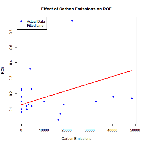
# --- Partial effect plots for each predictor in ROE model ---

# 1. Carbon Emissions vs ROE
plot(train$carbon_emissions, train$roe,
     xlab = "Carbon Emissions", ylab = "ROE",
     main = "Effect of Carbon Emissions on ROE",
     pch = 19, col = "blue")

emm_em <- data.frame(
  carbon_emissions = seq(min(train$carbon_emissions, na.rm = TRUE),
                         max(train$carbon_emissions, na.rm = TRUE),
                         length.out = 100),
  energy_consumption = mean(train$energy_consumption, na.rm = TRUE),
  employee_turnover  = mean(train$employee_turnover, na.rm = TRUE),
  industry_type      = train$industry_type[1], # pick one level as baseline
  ceo_gender         = train$ceo_gender[1],
  year               = mean(train$year, na.rm = TRUE)
)

lines(emm_em$carbon_emissions,
      predict(model_roe, newdata = emm_em),
      col = "red", lwd = 2)

legend("topleft", legend = c("Actual Data", "Fitted Line"),
       col = c("blue","red"), pch = c(19, NA), lty = c(NA,1))
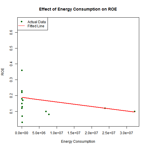
# 2. Energy Consumption vs ROE
plot(train$energy_consumption, train$roe,
     xlab = "Energy Consumption", ylab = "ROE",
     main = "Effect of Energy Consumption on ROE",
     pch = 19, col = "darkgreen")

emm_en <- data.frame(
  carbon_emissions   = mean(train$carbon_emissions, na.rm = TRUE),
  energy_consumption = seq(min(train$energy_consumption, na.rm = TRUE),
                           max(train$energy_consumption, na.rm = TRUE),
                           length.out = 100),
  employee_turnover  = mean(train$employee_turnover, na.rm = TRUE),
  industry_type      = train$industry_type[1],
  ceo_gender         = train$ceo_gender[1],
  year               = mean(train$year, na.rm = TRUE)
)

lines(emm_en$energy_consumption,
      predict(model_roe, newdata = emm_en),
      col = "red", lwd = 2)

legend("topleft", legend = c("Actual Data", "Fitted Line"),
       col = c("darkgreen","red"), pch = c(19, NA), lty = c(NA,1))
# 3. Employee Turnover vs ROE
plot(train$employee_turnover, train$roe,
     xlab = "Employee Turnover", ylab = "ROE",
     main = "Effect of Employee Turnover on ROE",
     pch = 19, col = "purple")

emm_to <- data.frame(
  carbon_emissions   = mean(train$carbon_emissions, na.rm = TRUE),
  energy_consumption = mean(train$energy_consumption, na.rm = TRUE),
  employee_turnover  = seq(min(train$employee_turnover, na.rm = TRUE),
                           max(train$employee_turnover, na.rm = TRUE),
                           length.out = 100),
  industry_type      = train$industry_type[1],
  ceo_gender         = train$ceo_gender[1],
  year               = mean(train$year, na.rm = TRUE)
)

lines(emm_to$employee_turnover,
      predict(model_roe, newdata = emm_to),
      col = "red", lwd = 2)

legend("topleft", legend = c("Actual Data", "Fitted Line"),
       col = c("purple","red"), pch = c(19, NA), lty = c(NA,1))
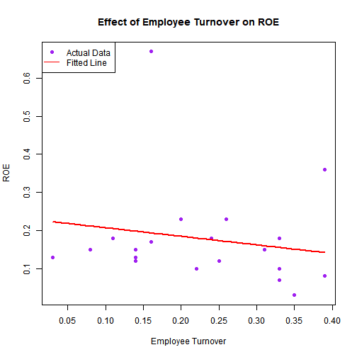
-
Pooled regression statistically valid but predictive accuracy remains weak.
-
Useful for identifying directional patterns (-turnover -> -ROE ; +emissions -> -ROE).
-
Confirms that external factors (market shocks, policies, R&D) drive much of the unexplained variation.
7) Conclusion
-
Our analysis linked sustainability metrics such as emissions, energy use and turnover with financial performance such as ROE/ROA across 10 companies over 5 years.
-
Company-level models failed due to very limited data (4–5 years per firm), showing why data depth matters in predictive analytics.
-
Pooled regression models were statistically valid but had weak predictive accuracy, highlighting the complex nature of ROE.
-
Despite poor prediction, the models provided directional insights:
-
Clustering analysis grouped firms into: efficient & profitable, underperformers, and transitioners — offering a method for strategic benchmarking.
8) Use of AI declaration
Declaration: AI tools were used only for grammatical refinement, formatting and pretty tables and graphs. All analysis, data preparation, modeling choices, and interpretations are original work.
9) Data sources declaration
-
Annual reports sourced from NSE India webpage
-
Sustainability reports also sourced from NSE India Webpage
-
Ratios through Dion Solutions Ltd. Available on MoneyControl
10) Blog link
https://proplayerplayz.github.io
]]>