Market Segmentation
1. Introduction
This document will perform Market Segmentation Analysis on the data provided by KTC. We will be looking into importing and performing cluster analysis on the data to find useful patterns in Customer data.
2. Descriptive Mining
We are going to explore the data and find the patterns and do the segmentation.
2.1. Data Exploration
We have information regarding 30 customers of KTC Company. We have details of their Age, Income, Marital Status, No. of Children and their financial status in the means of whether they have a mortgage loan and other loans.
## # A tibble: 30 × 7
##      Age Female Income Married Children  Loan Mortgage
##    <dbl>  <dbl>  <dbl>   <dbl>    <dbl> <dbl>    <dbl>
##  1    48      1 17546        0        1     0        0
##  2    40      0 30085.       1        3     1        1
##  3    51      1 16575.       1        0     1        0
##  4    23      1 20375.       1        3     0        0
##  5    57      1 50576.       1        0     0        0
##  6    57      1 37870.       1        2     0        0
##  7    22      0  8877.       0        0     0        0
##  8    58      0 24947.       1        0     1        0
##  9    37      1 25304.       1        2     1        0
## 10    54      0 24212.       1        2     1        0
## # ℹ 20 more rows
##
## Data frame:crs$dataset[, c(crs$input, crs$risk, crs$target)]	30 observations and 7 variables    Maximum # NAs:0
##
##
##          Storage
## Age       double
## Female    double
## Income    double
## Married   double
## Children  double
## Loan      double
## Mortgage  double
##       Age            Female           Income         Married       Children           Loan           Mortgage
##  Min.   :22.00   Min.   :0.0000   Min.   : 8877   Min.   :0.0   Min.   :0.0000   Min.   :0.0000   Min.   :0.0
##  1st Qu.:37.25   1st Qu.:0.0000   1st Qu.:18166   1st Qu.:1.0   1st Qu.:0.0000   1st Qu.:0.0000   1st Qu.:0.0
##  Median :47.00   Median :1.0000   Median :24241   Median :1.0   Median :0.5000   Median :0.0000   Median :0.0
##  Mean   :45.97   Mean   :0.5667   Mean   :28012   Mean   :0.8   Mean   :0.9333   Mean   :0.4333   Mean   :0.4
##  3rd Qu.:56.75   3rd Qu.:1.0000   3rd Qu.:35923   3rd Qu.:1.0   3rd Qu.:2.0000   3rd Qu.:1.0000   3rd Qu.:1.0
##  Max.   :66.00   Max.   :1.0000   Max.   :59804   Max.   :1.0   Max.   :3.0000   Max.   :1.0000   Max.   :1.0
2.1.1. Age
## crs$dataset["Age"]
##
##  1  Variables      30  Observations
## ------------------------------------------------------------------------------------------------------------------------------------
## Age
##        n  missing distinct     Info     Mean  pMedian      Gmd      .05      .10      .25      .50      .75      .90      .95
##       30        0       23    0.998    45.97     46.5    15.12    22.45    26.60    37.25    47.00    56.75    61.10    64.20
##
## lowest : 22 23 27 31 36, highest: 57 58 61 62 66
## ------------------------------------------------------------------------------------------------------------------------------------
2.1.2. Female (Gender Column
## crs$dataset["Female"]
##
##  1  Variables      30  Observations
## ------------------------------------------------------------------------------------------------------------------------------------
## Female
##        n  missing distinct     Info      Sum     Mean
##       30        0        2    0.737       17   0.5667
##
## ------------------------------------------------------------------------------------------------------------------------------------
2.1.3. Income
## crs$dataset["Income"]
##
##  1  Variables      30  Observations
## ------------------------------------------------------------------------------------------------------------------------------------
## Income
##        n  missing distinct     Info     Mean  pMedian      Gmd      .05      .10      .25      .50      .75      .90      .95
##       30        0       30        1    28012    25590    14919    13945    15716    18166    24241    35923    51039    56676
##
## lowest : 8877.07 12640.3 15538.8 15735.8 16497.3, highest: 41034   50576.3 55204.7 57880.7 59803.9
## ------------------------------------------------------------------------------------------------------------------------------------
2.1.4. Marriage
## crs$dataset["Married"]
##
##  1  Variables      30  Observations
## ------------------------------------------------------------------------------------------------------------------------------------
## Married
##        n  missing distinct     Info      Sum     Mean
##       30        0        2    0.481       24      0.8
##
## ------------------------------------------------------------------------------------------------------------------------------------
2.1.5. Children
## crs$dataset["Children"]
##
##  1  Variables      30  Observations
## ------------------------------------------------------------------------------------------------------------------------------------
## Children
##        n  missing distinct     Info     Mean  pMedian      Gmd
##       30        0        4    0.858   0.9333        1    1.163
##
## Value          0     1     2     3
## Frequency     15     5     7     3
## Proportion 0.500 0.167 0.233 0.100
##
## For the frequency table, variable is rounded to the nearest 0
## ------------------------------------------------------------------------------------------------------------------------------------
2.1.6. Loan
## crs$dataset["Loan"]
##
##  1  Variables      30  Observations
## ------------------------------------------------------------------------------------------------------------------------------------
## Loan
##        n  missing distinct     Info      Sum     Mean
##       30        0        2    0.737       13   0.4333
##
## ------------------------------------------------------------------------------------------------------------------------------------
2.1.7. Mortgage
## crs$dataset["Mortgage"]
##
##  1  Variables      30  Observations
## ------------------------------------------------------------------------------------------------------------------------------------
## Mortgage
##        n  missing distinct     Info      Sum     Mean
##       30        0        2    0.721       12      0.4
##
## ------------------------------------------------------------------------------------------------------------------------------------
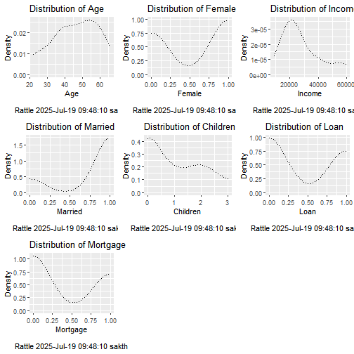
2.1.8. Distributions
# Generate the plot.

p01 <- crs %>%
  with(dataset[,]) %>%
  dplyr::select(Age) %>%
  ggplot2::ggplot(ggplot2::aes(x=Age)) +
  ggplot2::geom_density(lty=3) +
  ggplot2::xlab("Age\n\nRattle 2025-Jul-19 09:48:10 sakth") +
  ggplot2::ggtitle("Distribution of Age") +
  ggplot2::labs(y="Density")

# Use ggplot2 to generate histogram plot for Female

# Generate the plot.

p02 <- crs %>%
  with(dataset[,]) %>%
  dplyr::select(Female) %>%
  ggplot2::ggplot(ggplot2::aes(x=Female)) +
  ggplot2::geom_density(lty=3) +
  ggplot2::xlab("Female\n\nRattle 2025-Jul-19 09:48:10 sakth") +
  ggplot2::ggtitle("Distribution of Female") +
  ggplot2::labs(y="Density")

# Use ggplot2 to generate histogram plot for Income

# Generate the plot.

p03 <- crs %>%
  with(dataset[,]) %>%
  dplyr::select(Income) %>%
  ggplot2::ggplot(ggplot2::aes(x=Income)) +
  ggplot2::geom_density(lty=3) +
  ggplot2::xlab("Income\n\nRattle 2025-Jul-19 09:48:10 sakth") +
  ggplot2::ggtitle("Distribution of Income") +
  ggplot2::labs(y="Density")

# Use ggplot2 to generate histogram plot for Married

# Generate the plot.

p04 <- crs %>%
  with(dataset[,]) %>%
  dplyr::select(Married) %>%
  ggplot2::ggplot(ggplot2::aes(x=Married)) +
  ggplot2::geom_density(lty=3) +
  ggplot2::xlab("Married\n\nRattle 2025-Jul-19 09:48:10 sakth") +
  ggplot2::ggtitle("Distribution of Married") +
  ggplot2::labs(y="Density")

# Use ggplot2 to generate histogram plot for Children

# Generate the plot.

p05 <- crs %>%
  with(dataset[,]) %>%
  dplyr::select(Children) %>%
  ggplot2::ggplot(ggplot2::aes(x=Children)) +
  ggplot2::geom_density(lty=3) +
  ggplot2::xlab("Children\n\nRattle 2025-Jul-19 09:48:10 sakth") +
  ggplot2::ggtitle("Distribution of Children") +
  ggplot2::labs(y="Density")

# Use ggplot2 to generate histogram plot for Loan

# Generate the plot.

p06 <- crs %>%
  with(dataset[,]) %>%
  dplyr::select(Loan) %>%
  ggplot2::ggplot(ggplot2::aes(x=Loan)) +
  ggplot2::geom_density(lty=3) +
  ggplot2::xlab("Loan\n\nRattle 2025-Jul-19 09:48:10 sakth") +
  ggplot2::ggtitle("Distribution of Loan") +
  ggplot2::labs(y="Density")

# Use ggplot2 to generate histogram plot for Mortgage

# Generate the plot.

p07 <- crs %>%
  with(dataset[,]) %>%
  dplyr::select(Mortgage) %>%
  ggplot2::ggplot(ggplot2::aes(x=Mortgage)) +
  ggplot2::geom_density(lty=3) +
  ggplot2::xlab("Mortgage\n\nRattle 2025-Jul-19 09:48:10 sakth") +
  ggplot2::ggtitle("Distribution of Mortgage") +
  ggplot2::labs(y="Density")

# Display the plots.

gridExtra::grid.arrange(p01, p02, p03, p04, p05, p06, p07)
2.2. Dendrogram
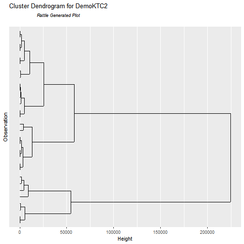
Observing the above dendrogram we can observe that
2.3. Elbow Method
# Elbow method for finding the no of clusters
library(factoextra)
## Welcome! Want to learn more? See two factoextra-related books at https://goo.gl/ve3WBa
fviz_nbclust(crs$dataset[, c(1:7)], kmeans, method = "wss") +
  labs(subtitle = "Elbow Method")
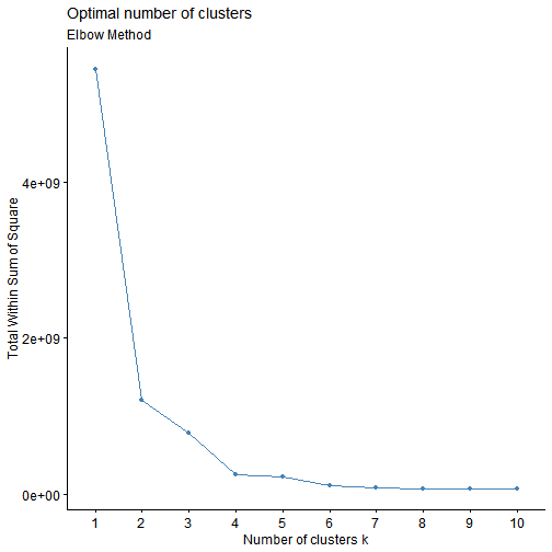
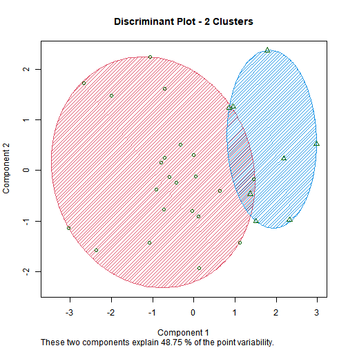
We can observe that when the no. of clusters is 2 there is a sharp change in the total within sum of squares. This shows that 2 is the optimal no. of clusters to have for this dataset
3. Segmentation and Clustering
Clustering is a method of grouping the observation based on their similarities. We use distance measures for assessing the dissimilarity among the observations. There are many measures of distance including Euclidean, Manhattan etc, Similarly we have different types of clustering algorithms such as K Means, Hierarchical, BiClustering etc. We will begin with Hierarchical clustering as part of our data exploration analysis.
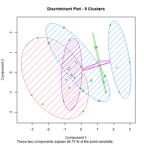
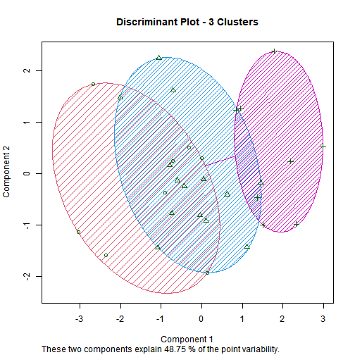
3.1. Hierarchical Clustering
No. of Clusters = 5
No. of Clusters = 4
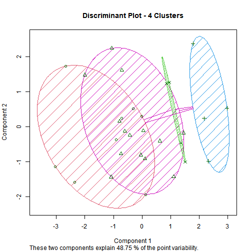
No. of Clusters = 3
No. of Clusters = 2
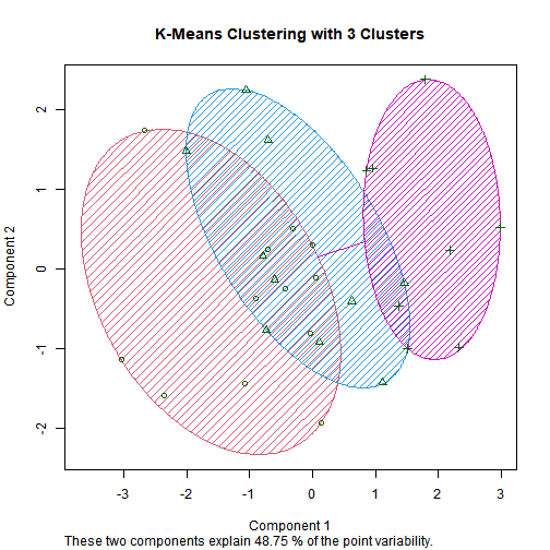
3.2. K-means Clustering
## [1] "12 10 8"
##          Age       Female       Income      Married     Children         Loan     Mortgage
## 4.596667e+01 5.666667e-01 2.801187e+04 8.000000e-01 9.333333e-01 4.333333e-01 4.000000e-01
##      Age    Female   Income   Married Children Loan  Mortgage
## 1 37.000 0.5833333 16826.18 0.6666667    1.000 0.25 0.4166667
## 2 47.200 0.5000000 25661.02 0.8000000    1.100 0.80 0.4000000
## 3 57.875 0.6250000 47728.97 1.0000000    0.625 0.25 0.3750000
## [1] 131352595 61338314 586111857
4. Conclusion
We have successfully explored the data and performed the appropriate clustering methods to identify the pattern in the data.
From this we can see the formed clusters clearly, and we can say that all the data points within each cluster are significantly similar to each other. From this we can do various analysis like classifying a new entry to the dataset or identifying largest common cluster to find the most common type of customers.